Building a Better Search Engine for the Allen Institute for Artificial Intelligence

 

Note: this blog post first appeared elsewhere and is reproduced here in a slightly altered format.

2020 is the year of search for Semantic Scholar (S2), a free, AI-powered research tool for scientific literature, based at the Allen Institute for AI. One of S2's biggest endeavors this year is to improve the relevance of our search engine, and my mission was to figure out how to use about three years of search log data to build a better search ranker.

We now have a search engine that provides more relevant results to users, but at the outset I underestimated the complexity of getting machine learning to work well for search. “No problem,” I thought to myself, “I can just do the following and succeed thoroughly in 3 weeks”:

1. Get all of the search logs.
2. Do some feature engineering.
3. Train, validate, and test a great machine learning model.
4. Deploy.

Although this is what seems to be established practice in the search engine literature, many of the experiences and insights from the hands-on work of actually making search engines work is often not published for competitive reasons. Because AI2 is focused on AI for the common good, they make a lot of our technology and research open and free to use. In this post, I’ll provide a “tell-all” account of why the above process was not as simple as I had hoped, and detail the following problems and their solutions:

1. The data is absolutely filthy and requires careful understanding and filtering.
2. Many features improve performance during model development but cause bizarre and unwanted behavior when used in practice.
3. Training a model is all well and good, but choosing the correct hyperparameters isn’t as simple as optimizing nDCG on a held-out test set.
4. The best-trained model still makes some bizarre mistakes, and posthoc correction is needed to fix them.
5. Elasticsearch is complex, and hard to get right.

Along with this blog post and in the spirit of openness, S2 is also releasing the complete Semantic Scholar search reranker model that is currently running on www.semanticscholar.org, as well as all of the artifacts you need to do your own reranking. Check it out here: https://github.com/allenai/s2search

Let me start by briefly describing the high-level search architecture at Semantic Scholar. When one issues a search on Semantic Scholar, the following steps occur:

1. Your search query goes to Elasticsearch (S2 has almost ~190M papers indexed).
2. The top results (S2 uses 1000 currently) are reranked by a machine learning ranker.

S2 has recently improved both (1) and (2), but this blog post is primarily about the work done on (2). The model used was a LightGBM ranker with a LambdaRank objective. It’s very fast to train, fast to evaluate, and easy to deploy at scale. It’s true that deep learning has the potential to provide better performance, but the model twiddling, slow training (compared to LightGBM), and slower inference are all points against it.

The data has to be structured as follows. Given a query q, ordered results set R = [r_1, r_2, …, r_M], and number of clicks per result C = [c_1, c_2, …, c_M], one feeds the following input/output pairs as training data into LightGBM:

f(q, r_1), c_1

f(q, r_2), c_2

…

f(q, r_m), c_m

Where f is a featurization function. We have up to m rows per query, and LightGBM optimizes a model such that if c_i > c_j then model(f(q, r_i)) > model(f(q, r_j)) for as much of the training data as possible.

One technical point here is that you need to correct for position bias by weighting each training sample by the inverse propensity score of its position. We computed the propensity scores by running a random position swap experiment on the search engine results page.

Feature engineering and hyper-parameter optimization are critical components to making this all work. We’ll return to those later, but first I’ll discuss the training data and its difficulties.

Machine learning wisdom 101 says that “the more data the better,” but this is an oversimplification. The data has to be relevant, and it’s helpful to remove irrelevant data. We ended up needing to remove about one-third of our data that didn’t satisfy a heuristic “does it make sense” filter.

What does this mean? Let’s say the query is Aerosol and Surface Stability of SARS-CoV-2 as Compared with SARS-CoV-1 and the search engine results page (SERP) returns with these papers:

1. Aerosol and Surface Stability of SARS-CoV-2 as Compared with SARS-CoV-1
2. The proximal origin of SARS-CoV-2
3. SARS-CoV-2 Viral Load in Upper Respiratory Specimens of Infected Patients
4. …

Another example: let’s say the user searches for deep learning, and the search engine results page comes back with papers with these years and citations:

1. Year = 1990, Citations = 15000
2. Year = 2000, Citations = 10000
3. Year = 2015, Citations = 5000

And now the click is on position (2). For the sake of argument, let’s say that all 3 papers are equally “about” deep learning; i.e. they have the phrase deep learning appearing in the title/abstract/venue the same number of times. Setting aside topicality, we believe that academic paper importance is driven by both recency and citation count, and here the user has clicked on neither the most recent paper nor the most cited. This is a bit of a straw man example, e.g., if number (3) had zero citations then many readers might prefer number (2) to be ranked first. Nevertheless, taking the above two examples as a guide, the filters used to remove “nonsensical” data checked the following conditions for a given triple (q, R, C):

1. Are all of the clicked papers more cited than the unclicked papers?
2. Are all of the clicked papers more recent than the unclicked papers?
3. Are all of the clicked papers more textually matched for the query in the title?
4. Are all of the clicked papers more textually matched for the query in the author field?
5. Are all of the clicked papers more textually matched for the query in the venue field?

I require that an acceptable training example satisfy at least one of these 5 conditions. Each condition is satisfied when all of the clicked papers have a higher value (citation number, recency, fraction of match) than the maximum value among the unclicked. You might note that abstract is not in the above list; including or excluding it didn’t make any practical difference.

As mentioned above, this kind of filter removes about one-third of all (query, results) pairs, and provides about a 10% to 15% improvement in our final evaluation metric, which is described in more detail in a later section. Note that this filtering occurs after suspected bot traffic has already been removed.

We generated a feature vector for each (query, result) pair, and there were 22 features in total. The first version of the featurizer produced 90 features, but most of these were useless or harmful, once again confirming the hard-won wisdom that machine learning algorithms often work better when you do some of the work for them.

The most important features involve finding the longest subsets of the query text within the paper’s title, abstract, venue, and year fields. To do so, we generate all possible ngrams up to length 7 from the query, and perform a regex search inside each of the paper’s fields. Once we have the matches, we can compute a variety of features. Here is the final list of features grouped by paper field.

• title_fraction_of_query_matched_in_text
• title_mean_of_log_probs
• title_sum_of_log_probs*match_lens
• abstract_fraction_of_query_matched_in_text
• abstract_mean_of_log_probs
• abstract_sum_of_log_probs*match_lens
• abstract_is_available
• venue_fraction_of_query_matched_in_text
• venue_mean_of_log_probs
• venue_sum_of_log_probs*match_lens
• sum_matched_authors_len_divided_by_query_len
• max_matched_authors_len_divided_by_query_len
• author_match_distance_from_ends
• paper_year_is_in_query
• paper_oldness
• paper_n_citations
• paper_n_key_citations
• paper_n_citations_divided_by_oldness
• fraction_of_unquoted_query_matched_across_all_fields
• sum_log_prob_of_unquoted_unmatched_unigrams
• fraction_of_quoted_query_matched_across_all_fields
• sum_log_prob_of_quoted_unmatched_unigrams

A few of these features require further explanation. Visit the appendix at the end of this post for more detail. All of the featurization happens here if you want the gory details.

To get a sense of how important all of these features are, below is the SHAP value plot for the model that is currently running in production.

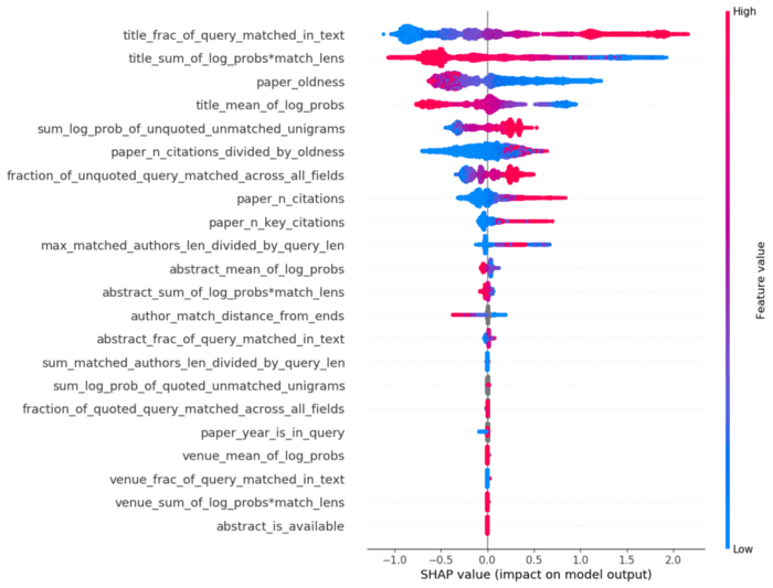
In case you haven’t seen SHAP plots before, they’re a little tricky to read. The SHAP value for sample i and feature j is a number that tells you, roughly, “for this sample i, how much does this feature j contribute to the final model score.” For our ranking model, a higher score means the paper should be ranked closer to the top. Each dot on the SHAP plot is a particular (query, result) click pair sample. The color corresponds to that feature’s value in the original feature space. For example, we see that the title_fraction_of_query_matched_in_text feature is at the top, meaning it is the feature that has the largest sum of the (absolute) SHAP values. It goes from blue on the left (low feature values close to 0) to red on the right (high feature values close to 1), meaning that the model has learned a roughly linear relationship between how much of the query was matched in the title and the ranking of the paper. The more the better, as one might expect.

A few other observations:

• A lot of the relationships look monotonic, and that’s because they approximately are: LightGBM lets you specify univariate monotonicity of each feature, meaning that if all other features are held constant, the output score must go up in a monotonic way if the feature goes up/down (up and down can be specified).
• Knowing both how much of the query is matched and the log probabilities of the matches is important and not redundant.
• The model learned that recent papers are better than older papers, even though there was no monotonicity constraint on this feature (the only feature without such a constraint). Academic search users like recent papers, as one might expect!
• When the color is gray, this means the feature is missing — LightGBM can handle missing features natively, which is a great bonus.
• Venue features look very unimportant, but this is only because a small fraction of searches are venue-oriented. These features should not be removed.

As you might expect, there are many small details about these features that are important to get right. It’s beyond the scope of this blog post to go into those details here, but if you’ve ever done feature engineering you’ll know the drill:

1. Design/tweak features.
2. Train models.
3. Do error analysis.
4. Notice bizarre behavior that you don’t like.
5. Go back to (1) and adjust.
6. Repeat.

Nowadays, it’s more common to do this cycle except replacing (1) with “design/tweak neural network architecture” and also add “see if models train at all” as an extra step between (1) and (2).

Another infallible dogma of machine learning is the training, validation/development, and test split. It’s extremely important, easy to get wrong, and there are complex variants of it (one of my favorite topics). The basic statement of this idea is:

1. Train on the training data.
2. Use the validation/development data to choose a model variant (this includes hyperparameters).
3. Estimate generalization performance on the test set.
4. Don’t use the test set for anything else ever.

This is important, but is often impractical outside of academic publication because the test data you have available isn’t a good reflection of the “real” in-production test data. This is particularly true for the case when you want to train a search model.

To understand why, let’s compare/contrast the training data with the “real” test data. The training data is collected as follows:

1. A user issues a query.
2. Some existing system (Elasticsearch + existing reranker) returns the first page of results.
3. The user looks at results from top to bottom (probably). They may click on some of the results. They may or may not see every result on this page. Some users go on to the second page of the results, but most don’t.

Even the best model sometimes made foolish-seeming ranking choices because that’s the nature of machine learning models. Many such errors are fixed with simple rule-based posthoc correction. Here’s a partial list of posthoc corrections to the model scores:

1. Quoted matches are above non-quoted matches, and more quoted matches are above fewer quoted matches.
2. Exact year match results are moved to the top.
3. For queries that are full author names (like Isabel Cachola), results by that author are moved to the top.
4. Results where all of the unigrams from the query are matched are moved to the top.

You can see the posthoc correction in the code here.

We ran an A/B test for a few weeks to assess the new reranker performance. Below is the result when looking at (average) total number of clicks per issued query.

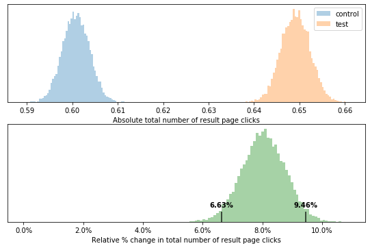
This tells us that people click about 8% more often on the search results page. But do they click on higher position results? We can check that by looking at the maximum reciprocal rank clicked per query. If there is no click, a maximum value of 0 is assigned.

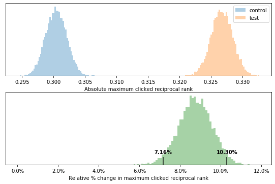
The answer is yes — the maximum reciprocal rank of the clicks went up by about 9%! For a more detailed sense of the click position changes here are histograms of the highest/maximum click position for control and test:

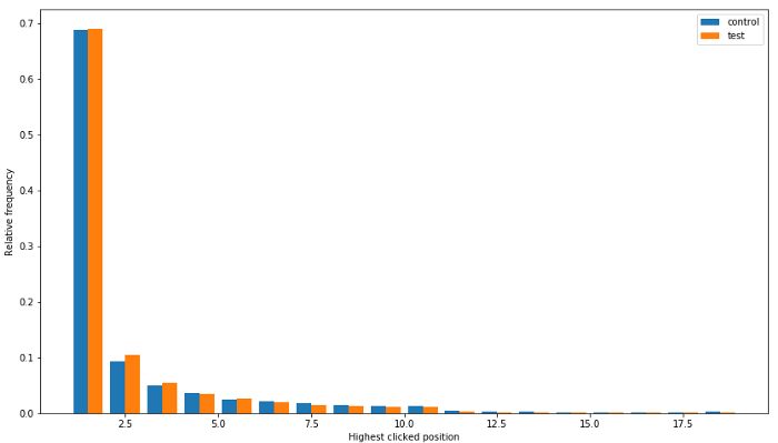
This histogram excludes non-clicks, and shows that most of the improvement occurred in positions 2, followed by position 3, and position 1.

This entire process took about 5 months, and would have been impossible without the help of a good portion of the Semantic Scholar team. In particular, I’d like to thank Doug Downey and Daniel King for tirelessly brainstorming with me, looking at countless prototype model results, and telling me how they were still broken but in new and interesting ways. I’d also like to thank Madeleine van Zuylen for all of the wonderful annotation work she did on this project, and Hamed Zamani for helpful discussions. Thanks as well to the engineers who took my code and magically made it work in production.

• *_fraction_of_query_matched_in_text — What fraction of the query was matched in this particular field?
• log_prob — Language model probability of the actual match. For example, if the query is deep learning for sentiment analysis, and the phrase sentiment analysis is the match, we can compute its log probability in a fast, low-overhead language model to get a sense of the degree of surprise. The intuition is that we not only want to know how much of the query was matched in a particular field, we also want to know if the matched text is interesting. The lower the probability of the match, the more interesting it should be. E.g. “preponderance of the viral load” is a much more surprising 4-gram than “they went to the store”. *_mean_of_log_probs is the average log probability of the matches within the field. We used KenLM as our language model instead of something BERT-like — it’s lightning fast which means we can call it dozens of times for each feature and are still able to featurize quickly-enough for running the Python code in production. (Big thanks to Doug Downey for suggesting this feature type and KenLM.)
• *_sum_of_log_probs*match_lens — Taking the mean log probability doesn’t provide any information about whether a match happens more than once. The sum benefits papers where the query text is matched multiple times. This is mostly relevant for the abstract.
• sum_matched_authors_len_divided_by_query_len — This is similar to the matches in title, abstract, and venue, but the matching is done one at a time for each of the paper authors. This feature has some additional trickery whereby we care more about last name matches than first and middle name matches, but not in an absolute way. You might run into some unfortunate search results where papers with middle name matches are ranked above those with last name matches. This is a feature improvement TODO.
• max_matched_authors_len_divided_by_query_len — The sum gives you some idea of how much of the author field you matched overall, and the max tells you what the largest single author match is. Intuitively if you searched for Sergey Feldman, one paper may be by (Sergey Patel, Roberta Feldman) and another is by (Sergey Feldman, Maya Gupta), the second match is much better. The max feature allows the model to learn that.
• author_match_distance_from_ends — Some papers have 300 authors and you’re much more likely to get author matches purely by chance. Here we tell the model where the author match is. If you matched the first or last author, this feature is 0 (and the model learns that smaller numbers are important). If you match author 150 out of 300, the feature is 150 (large values are learned to be bad). An earlier version of the feature was simply len(paper_authors), but the model learned to penalize many-author papers too harshly.
• fraction_of_*quoted_query_matched_across_all_fields — Although we have fractions of matches for each paper field, it’s helpful to know how much of the query was matched when unioned across all fields so the model doesn’t have to try to learn how to add.
• sum_log_prob_of_unquoted_unmatched_unigrams — The log probabilities of the unigrams that were left unmatched in this paper. Here the model can figure out how to penalize incomplete matches. E.g. if you search for deep learning for earthworm identification the model may only find papers that don’t have the word deep OR don’t have the word earthworm. It will probably downrank matches that exclude highly surprising terms like earthworm assuming citation and recency are comparable.